Monte Carlo Methods
Sometimes it is impossible to assume complete knowledge of the environment. Monte Carlo methods require only experience, including sample sequences of states, actions, and rewards from actual or simulated interaction with an environment.
A model is still required, but it only needs to generate sample transitions, not the complete probability distributions of all possible transitions that is required for DP. This means, mcm does not need transition probabilities, like \(p(s',r|s,a)\).
Monte Carlo Methods (MCM) sample and average returns for each state-action pair, like the bandit methods sample and average rewards for each action. The main difference is that now there are multiple states, each acting like a different bandit problem and that the different bandit problems are interrelated.
Monte Carlo Prediction
To learn the state-value function for a given policy, given that the value of a state is the expected return starting from that state, the average of returns should converge to the expected value when more returns are observed.
For instance, to estimate \(v_\pi(s)\). Each occurence of state \(s\) in an episode is called a visit, the first-visit MC method estimates the value ast the average of the returns following first visits to \(s\), the every-visit MC method averages the returns following all visits to \(s\). Both converge as the number of visits goes to infinity, but every-visit MC is less straightforward.
- First visit MC \(G\leftarrow \text{return following the 1st occurence of }s\)
- Every visit MC
Blackjack experiment
Assume that player hits (request one more card) whenever his sum is not 20 or 21. Ace can be counted as 1 or 11. In this case, the ace is suppressed to 1 if the sum is greater than 20 or 21. If the sum is 20 or 21, the player sticks (stop). This is the player policy. The dealer never hits, and only the first card is shown.
The rewards of 1,-1 and 0 are given for winning, losing, and drawing respectively. The game ends when the player stops hitting.
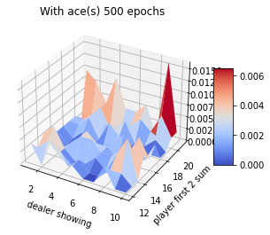
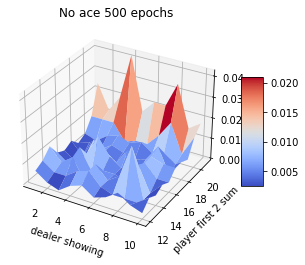
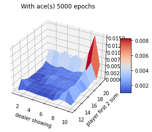
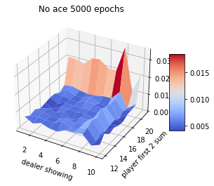
1. Although this game has complete knowledge of the environment, it would not be easy to apply DP methods, since they require the quantities \(p(s',r|s,a)\) and the expected rewards. 2. An important fact about MC methods is that the estimates for each state are independent. The estimate for one state does not build upon the estimate of any other state, as in the ase in DP. 3. The computational expense of estimating the value of a single state is independent of the number of states. This is an attractive pt of MC methods when one requires the value of only one or a subset of states.
MC Estimation of Action Values
With a model, state values are sufficient to determine a policy by looking ahead one step and choosing whichever action leading to the best combination of reward and next state. Without a model, values of action-state pairs are important.
The problem of policy evaluation based on policy evaluation of \(q_\pi(s,a)\) is that many state-action pairs may never be visited. To maintain exploration, the exploring starts can be adapted. It allows each episodes start in a state-action pair, and that every pair has a nonzero probability of being selected as the start.
MC Control
MC estimation can be used in generalized policy iteration (GPI) \(\pi\leftrightarrow q_\pi\).
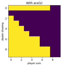
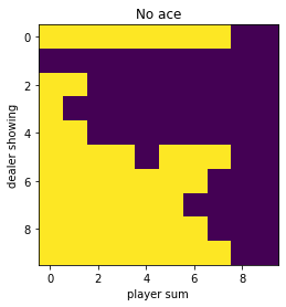
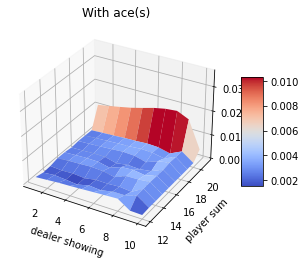
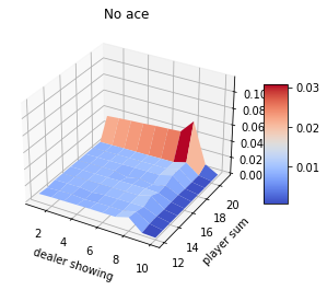
$$\pi(s)=\arg\max_a q(s,a)$$ $$q_{\pi_k}(s,\pi_k(s)) = v_{\pi_k}(s)$$In MC ES, all returns for each state-action pair are accumulated and averaged, irrespective of what policy was in force when they were observed. It may not converge, but if it did, the value function would eventually converge to the value function for that policy. Stability is achieved only when both policy and value are optimal. Convergence may seem inevitable, but has not yet been proved.
MC Control without Exploring Starts
To ensure all actions are selected infinitely, we need the agent to continue the selection, not with exploring starts.
- On policy methods: attempt to evaluate/improve the policy thats used to make decisions. (above example)
- Off policy methods: evaluate or improve a policy different from that used to generate the data.
In on-policy control methods the policy is generally soft, i.e. \(\pi(a|s)>0\) for all \(s\in\mathcal{S}\) and all \(a\in\mathcal{A}\), gradually shifted closer to a deterministic optimal policy.
\(\epsilon\)-greedy on policy
Most of the time choose an action maximizing the estimated action value, but sometime select an action at random.