Multi-arm Bandits

Action-Value Methods

The true value of action $a$ as $q(a)$, and the estimated value of t-th time step as $Q_t(a)$. With the sample-average method, the true value of an action is the mean reward received when that action is selected.

$$Q_t(a) = \frac{R_1+R_2+\cdots+R_{N_t(a)}}{N_t(a)}$$

Simplest action selection rule is with the highest estimated action value, the greedy action is given by,

$$A_t = \arg\max_aQ_t(a)$$

Alternative is to introduce $\epsilon$ which is a small probability to select randomly from amongst all the actions with equal probability. This is called $\epsilon-greedy$ method.

Experiment

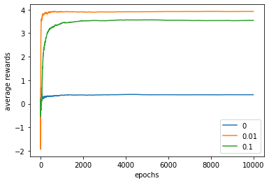
Estimate the convergence by the settings, $T=2000$, $q(a)\sim\mathcal{N}(0,1)$, $a^* = \arg\max_a q(a)$(true action, true action value). In the real world, select greedy or not by $\mathbb{U}(0,1)$,

$$R_t = q(A_t)+\mathcal{N}(0,1) \\ A_t = \begin{cases}\arg\max_a Q_t(a),&\text{if }1-\epsilon\\ \mathbb{U}(0,1),&\text{if }\epsilon \end{cases}$$


def nArmBandit(qa,ep,T=1000):
    allq = 5*np.ones((10,1))
    alln = np.zeros((10,1))
    sumr = 0
    pltavgr = [0]
    for i in range(1,T):
        greedy = (np.random.rand(1)<=1-ep)
        if greedy:
            a = np.argmax(allq)
        else:
            a = np.random.choice(10)
        alln[a] += 1
        r = trueQa[a]+np.random.randn(1)
        allq[a] += r/alln[a]
        sumr += r
        pltavgr.append(sumr/i)
    return pltavgr

The $\epsilon$-greedy method is better when the reward variance is greater. With noisier rewards it takes more exploration to find the optimal action.

Keeping track of each action and reward at a give time can lead to a problem of memory and computational requirements. Alternatively, the action value and k value are only necessary in another implementation,

$$ \begin{align*} Q_{k+1}&=\frac{1}{k}\sum^k_{i=1}R_i=\frac{1}{k}(R_k+\sum^{k-1}_{i=1}R_i)\\ &=\frac{1}{k}(R_k+(k-1)Q_k)\\ &=Q_k+\frac{1}{k}(R_k-Q_k)=Q_k+\alpha(R_k-Q_k) \end{align*} $$

This update rule is a common form later on. NewEstimate $\leftarrow$ OldEstimate + StepSize[Target-OldEstimate].

Exponential recency weight average,

$$Q_{k+1}=(1-\alpha)^kQ_1 + \sum^k_{i=1}\alpha(1-\alpha)^{k-i}R_i$$

The sample average method guarantees to converge for only one action, but not for all choices of the sequence $\{\alpha_k(a)\}$. Another stochastic approximation theory gives the conditions requirement to assure convergence with probability 1:

$$\sum^\infty_{k=1}\alpha_k(a) = \infty \quad\text{and}\quad \sum^\infty_{k=1}\alpha^2_k(a)\lt\infty$$

Therefore, a constant step size never converges, as the second requirement does not meet.

Optimistic Initial Values

Bias exists if not all actions have been selected at least once. Initial action values can be used as a simple way of encouraging exploration.

Upper-Confidence Bound Action Selection

The greedy actions are those that look best at present. $\epsilon$-greedy forces the non-greedy action to be tried, but no preference for those that are uncertain.

It is better to select among the non-greedy actions according to their potential based on their variance or uncertainty. So the one without being explored should be selected.

$$ A_t = \arg\max_a [ Q_t(a) + c\sqrt{\frac{\ln t}{N_t(a)}} ] $$ where $c=2$ is the degree of exploration.

Gradient Bandits

Learning a numerical preference $H_t(a)$ for each action $a$. The larger the preference, the more often that action is taken. The relative preference of one action over another is defined as a softmax distribution (gibbs/boltzmann),

$$Pr\{A_t=a\}=\frac{e^{H_t(a)}}{\sum^n_{b=1}e^{H_t(b)}}=\pi_t(a)$$

Natural learning algorithm (from stochastic gradient ascent),

$$H_{t+1}(A_t) = H_t(A_t)+\alpha(R_t-\bar{R}_t)(1-\pi_t(A_t)) $$

For $\forall a\neq A_t$,